

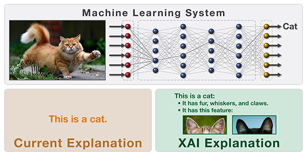
Explainable ARTIFICIAL INTELLIGENCE (XAI) is a model that could in the future explain the mechanisms behind machine learning algorithms.
Many solutions that use AI algorithms are a kind of “black box” – often not only end users, but also the developers themselves cannot determine exactly how the machine learning model came to certain conclusions during the processing of the original data.

Understanding the algorithms of artificial intelligence will allow developers to accurately assess the impact of input features on the output result of the model, identify biases and shortcomings associated with the operation of the model, as well as fine-tune and optimize THE AI.
For users, the explainability of the result of AI work is important in terms of understanding the reasons for the conclusions made by the model, and for experts – to explain those conclusions that at first glance have no basis.
The need for explainable artificial intelligence on the part of society is confirmed by such documents as Article 22 of the General Data Protection Regulation (EU) gives a person the right to demand an explanation of how the automated system made a decision that affects him; The Algorithmic Accountability Act (US) expressly requires companies to provide an assessment of the privacy or security risks posed by an automated decision-making system, as well as risks that contribute to inaccurate, unfair, biased or discriminatory decisions; The Equal Opportunity for Credit Act (US) establishes the possibility of explaining the reasons for obtaining or refusing a loan, which seems difficult when using artificial intelligence based on the “black box” and others.
The problem of explaining the work of artificial intelligence is dealt with by such large educational institutions as the University of Technology of Michigan (USA), Cornell University (USA), Carnegie Mellon University (USA), Duke University (USA), University of Edinburgh (UK), Bournemouth University (UK), University of London (UK), Norwegian University of Natural and Technical Sciences. Groups of scientists engaged in the study and development of this problem are allocated grants from governments and universities.
The Defense Advanced Research Projects Agency (DARPA) of the US Department of Defense, responsible for the development of new technologies, conducts the Explainable AI (XAI) program. Eleven XAI teams are exploring a wide range of methods and approaches for developing explainable models and effective explanation interfaces.
The national technology development programs of countries such as France, Norway, India, South Korea and others also talk about the need to develop XAI as an integral part of public policy.
The explainability of the model can be considered at all stages of the development of artificial intelligence, both for initially interpreted AI models (linear and logistic regression, decision trees, and others), and for models based on the “black box” (perceptron, convolutional and recurrent neural networks, long-term short-term memory network, and others).
For models that are difficult to interpret by users, the most popular in the scientific community a posteriori methods of explanation (explainability after modeling) are LIME, SHAP and LRP.
IBM, Microsoft, Google, and the open-source community provide users with toolkits and software packages for explainable artificial intelligence.
The development of XAI technologies is at an early stage – most of the methods are still under development, new combined methods appear, during the experiments some of the theories are criticized. The number and level of research participants involved indicate the importance of the topic under consideration.
XAI methods can be used to predict risks and threats in the dissemination of information, but the greatest effect of the technology can be obtained with the development of XAI methods, which identify various types of heterogeneous unstructured media materials. This should be taken into account when developing the conceptual architecture of the information systems of the department.
Tasks solved with the help of machine learning and artificial intelligence
All tasks solved with the help of machine learning (ML) and artificial intelligence (AI) belong to one of the following categories:
1) The regression problem is a prediction based on a sample of objects with various features. The output should be a real number.
2) The task of classification is to obtain a categorical response based on a set of features. It has a finite number of answers (usually in the format of “yes” or “no”).
3) The task of clustering is to distribute data into groups.
4) The task of reducing dimensionality is to reduce a large number of features to a smaller one (usually 2-3) for the convenience of their subsequent visualization.
5) The task of detecting anomalies is to identify deviations from standard cases. Similar to the classification task, but more difficult to learn.
Artificial intelligence/machine learning models are mathematical algorithms that, with the help of the contribution of a person (expert), are “trained” on data sets to reproduce the decision that the expert will make when analyzing the same data set. Having learned to reproduce the solution of the Expert Advisor, the model further functions independently, thus allowing you to automate the solution of problems. Ideally, the model should also justify its decision to help interpret the decision-making process.
Artificial Neural Networks
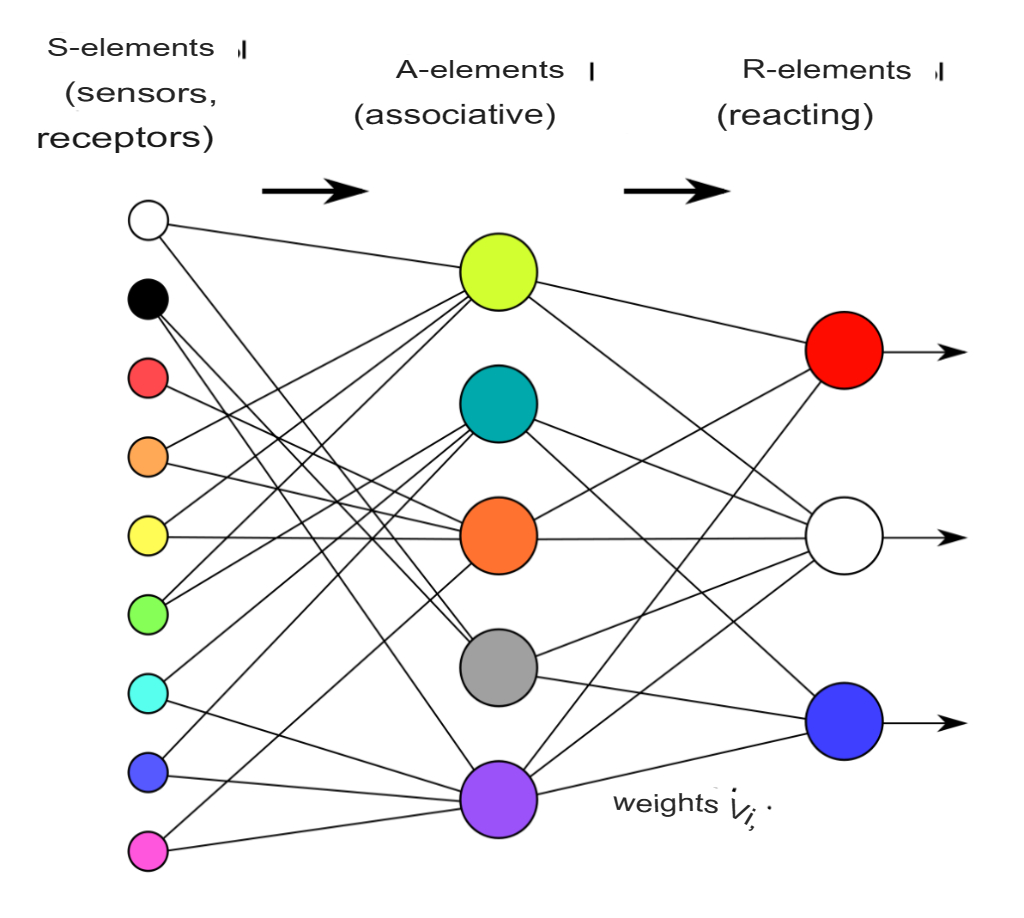
An artificial neural network (ANN) is a mathematical model, as well as its software or hardware embodiment, built on the principle of organization and functioning of biological neural networks. In general, the ANN may consist of several layers of the simplest processors (neurons), each of which performs some mathematical transformation (calculates the result of a mathematical function) over the input data and transmits the result to the next layer or to the output of the network.
ANNs solve the problems of pattern recognition, prediction, optimization, associative memory, and control.
Neurons of the input layer receive data from the outside (for example, from the sensors of the facial recognition system) and, after processing them, transmit signals through the synapses to the neurons of the next layer. Neurons of the second layer (it is called hidden, because it is not directly related to either the input or the output of the ANN) process the received signals and transmit them to the neurons of the output layer. Since we are talking about imitation of neurons, each input-level processor is associated with several hidden-level processors, each of which, in turn, is connected to several output-level processors. Such a simple ANN is capable of learning and can find simple relationships in the data. A more complex ANN model would have several hidden layers of neurons interspersed with layers that perform complex logical transformations. Each subsequent layer of the network looks for relationships in the previous one. Such ANNs are capable of deep (deep) learning (Fig. 1).
The perceptron is the simplest model of a neural network consisting of a single neuron. A neuron can have an arbitrary number of inputs, and one of them is usually identical to 1. This single input is called an offset. Each entrance has its own weight. When a signal enters the neuron, a weighted sum of signals is calculated, then an activation function is applied to the signal and the signal is transmitted to the output (Fig. 1). Such a simple network is able to solve a number of tasks: perform the simplest forecast, regression of data, etc., as well as simulate the behavior of simple functions. The main thing for the efficiency of this network is the linear data separability.
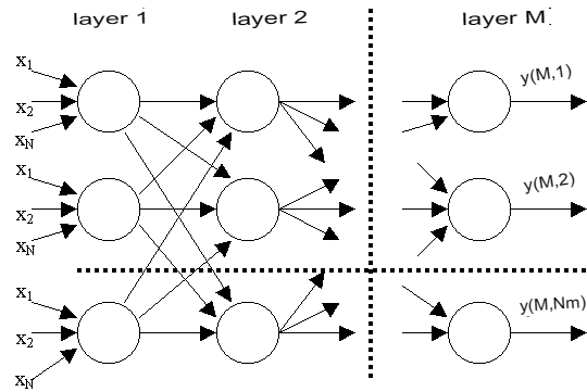
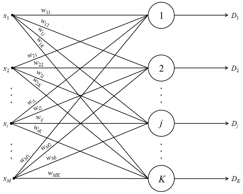
A multilayer perceptron is a generalization of a single-layer perceptron. A layer is a union of neurons; in diagrams, as a rule, layers are depicted as one vertical row (in some cases, the scheme can be rotated, and then the row will be horizontal). A multilayer perceptron consists of some set of input nodes (Fig. 2), several hidden layers of computational neurons, and an output layer.
Distinctive features of a multilayer perceptron:
- All neurons have a nonlinear activation function that is differentiable.
- The network achieves a high degree of connectivity using synaptic connections.
- A network has one or more hidden layers.
Such multilayer networks are also called deep. This network is needed to solve problems that the perceptron cannot cope with – in particular, linearly inseparable tasks. The multilayer perceptron is the only universal neural network, a universal approximator capable of solving any machine learning problem. That is why, if the researcher is not sure what kind of neural network is suitable for solving the task facing him, he first chooses a multilayer perceptron.
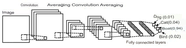
Convolutional neural network (CNN) is a network that processes the transmitted data not in whole, but in fragments. The data is processed sequentially, and then transmitted further through the layers. Convolutional neural networks consist of several types of layers: a convolutional layer, a subsampling layer, a layer of a fully connected network (when each neuron of one layer is connected to each neuron of the next). Convolution layers and subsampling (subsampling) alternate and can be repeated several times. Perceptrons are often added to the finite layers, which serve for subsequent data processing (Fig. 3).
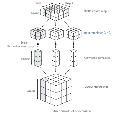
The essence of the convolution operation is that each fragment of the image is multiplied by the matrix (core) of the convolution element-by-element, and the result is summed up and recorded in a similar position of the output image to move from specific features of the image to more abstract details, and then to even more abstract ones, up to highlighting high-level concepts (is there anything you are looking for in the image).
Convolutional neural networks solve the following problems: classification, detection (search and definition of objects) and segmentation.
The described networks refer to direct distribution networks. Along with them, there are neural networks, the architectures of which have in their composition connections through which the signal propagates in the opposite direction.
Recurrent neural network (RNN) is a network whose connections between neurons form an oriented cycle, i.e. there are feedbacks in the network. In this case, information to neurons can be transmitted both from previous layers and from themselves from the previous iteration (delay) (Fig. 4).
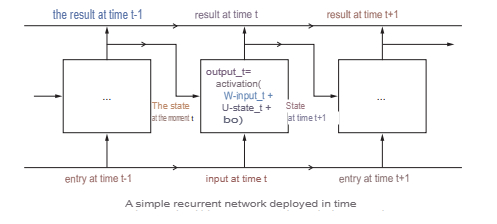
Network Specifications:
- Each connection has its own weight, which is also a priority.
- Nodes are divided into two types: input and hidden.
- The information in the neural network can be transmitted both in a straight line – layer by layer, and between neurons.
The peculiarity of the recurrent neural network is that it has “areas of attention”. This area allows you to specify the fragments of transmitted data that require enhanced processing.
Information in recurrent networks is lost over time at a rate dependent on activation functions. These networks are used in the recognition and processing of text data.
The Long short-term memory (LSTM) network is a special kind of recurrent neural network architecture capable of learning long-term dependencies. Therefore, the LSTM is suitable for predicting various changes using extrapolation (trend identification based on data), as well as in any tasks where the ability to “keep context” is important (Fig. 5).
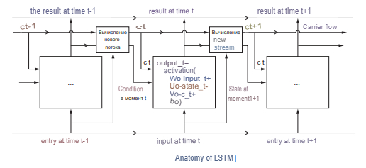
Any recurrent neural network has the form of a chain of repeating modules of a neural network. In an RNN, the structure of one such module is very simple, for example, it can be a single layer with a tanh activation function (hyperbolic tangent). The structure of the LSTM also resembles a chain, but instead of one layer of a neural network, it contains four, and these layers interact in a special way.
The first step in LSTM is to determine what information can be thrown out of the cell state. This decision is made by a sigmoidal layer called the forget gate layer.
The next step is to decide what new information will be stored in the cell state. This phase consists of two parts. First, a sigmoidal layer called an input layer gate determines which values to update. The tanh layer then builds a vector of new candidate values that can be added to the cell state.
Then the old values are replaced with new ones, after which the output data is calculated. First, the sigmoidal layer comes into play, which decides what information from the cell state should be output. The cell state values then pass through the tanh layer to output values from -1 to 1, and multiply with the output values of the sigmoidal layer, allowing only the required information to be output.
A self-organizing neural network (e.g., a Kohonnen network,
Figs. 6 and 7) is a neural network whose structure has one layer of neurons without bias coefficients (identical to single inputs). The process of learning the network takes place using the method of successive approximations. The neural network adapts to the patterns of input data, and not to the best value at the output. As a result of training, the network finds the area in which the best neuron is located, which in the end will have 1 at the output, and the rest of the neurons, the signal on which the signal turned out to be less – 0.
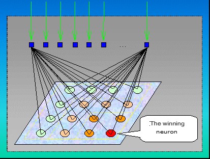
Rice. 7. Scheme of activation of neurons of Kohonnen networks
Such networks are often used in clustering and classification tasks.
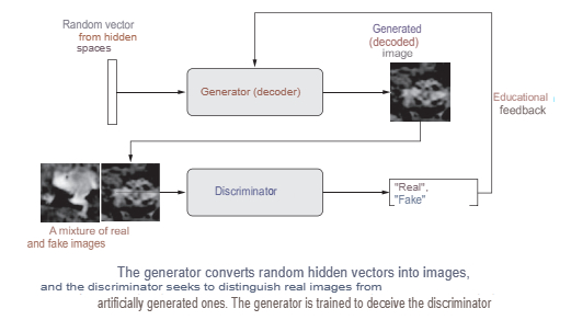
Generative adversarial network (GAN) is an architecture consisting of a generator and a discriminator configured to work against each other. GANs inherently mimic any distribution of data. GANs are trained to create structures similar to entities from the real world in the fields of images, music, speech, and prose (Fig. 8).
Discriminatory algorithms try to classify input data. Given the specifics of the data obtained, the networks try to determine the category to which the data belongs.
Generative algorithms try to match images to this category.
The steps that the GAN goes through are:
- The generator receives a random number and returns an image.
- This generated image is fed into the discriminator along with a stream of images taken from the actual dataset.
- The discriminator accepts both real and fake images and returns probabilities, numbers from 0 to 1, with 1 representing the genuine image and 0 representing the fake one.
Thus, GAN has a double feedback loop:
- The discriminator is in a loop with authentic images.
- The generator is in a loop along with the discriminator.
A discriminator is a standard convolutional network that can classify images fed to it using a binomial classifier that recognizes images as real or as fake. The generator is in a sense a reverse convolutional network: although a standard convolutional classifier takes an image and reduces its resolution to obtain a probability, the generator takes a random noise vector and converts it into an image. The former sifts out the data using downgrade sampling techniques such as maxpooling, and the latter generates new data.
Both networks try to optimize the objective function or loss function in a zero-sum game.
When building a model, first of all, there is a choice of the algorithm of its work, the most suitable for solving a specific problem.
Rationale for the use of explainable artificial intelligence (XAI)
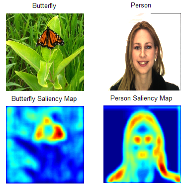
Deep learning models and neural networks work on the basis of hidden layers (i.e., there are several levels of mathematical processing and decision-making between the input data and the output result), but demonstrate the results better than the basic machine learning algorithms. The use of such models in areas with an increased level of responsibility for the decisions made led to the creation of the concept of explainable artificial intelligence, which explores methods for analyzing or supplementing AI models that make the internal logic and output of algorithms transparent and interpretable to humans (Fig. 9).
It is assumed that the explainability of AI will include three components: simulatability, decomposability, algorithmic transparency.
Simulation means the possibility of human analysis of the model; the most important criterion for simulation is the complexity of the model. Simple but extensive (with too many rules) rule-based systems do not meet this characteristic, whereas a single perceptron neural network falls into it.
Decomposability means the ability to explain each of the parts of the model (inputs, parameters, and outputs). Cumbersome functions do not meet this criterion.
Algorithmic transparency refers to the user’s ability to understand the process that the AI model follows in order to produce any given inference from its input data. A linear AI model is considered transparent because its error surface (a mathematical interpretation of the AI learning mechanism) is understandable and can be considered, giving the user enough knowledge about how the model will act in each situation they may encounter. In deep AI architectures, this does not happen, since the error surface can be opaque and cannot be fully observed, respectively, the solution must be approximated using heuristic optimization (for example, using stochastic gradient descent).
Explanations of AI algorithms can be presented in text or visual form.
Text explanations are a method of creating symbols that display the logic of an algorithm through semantic mapping.
Many of the visualization methods are accompanied by methods of reducing the dimensionality to simplify the understanding of the model by a person. Imaging techniques can be combined with other techniques to improve their understanding and are considered the most appropriate way to represent complex interactions between the variables involved in the model.
There are several different approaches to solving the problem of AI explainability.
Local explanations segment the solution space and provide explanations for less complex subspaces of solutions that are relevant to the entire model. These explanations can be formed using methods that explain part of the functioning of the entire system.
Example explanations involve extracting representative examples that capture the internal relationships and correlations detected by the data model being analyzed and relate to the result generated by a particular model.
Explanations through simplification collectively denote those methods in which an entire new AI system is rebuilt based on a trained AI model that needs to be explained. New AI typically tries to optimize its similarity to the original AI model, while reducing its complexity but maintaining the same level of performance.
Methods of a posteriori explanation of the relevance of features clarify the internal functioning of the model by calculating the relevance score for its controlled variables. These estimates quantify the effect (sensitivity) on the model output. Comparing the scores of different variables shows the weight that the model assigns to each of these variables when it obtains results.
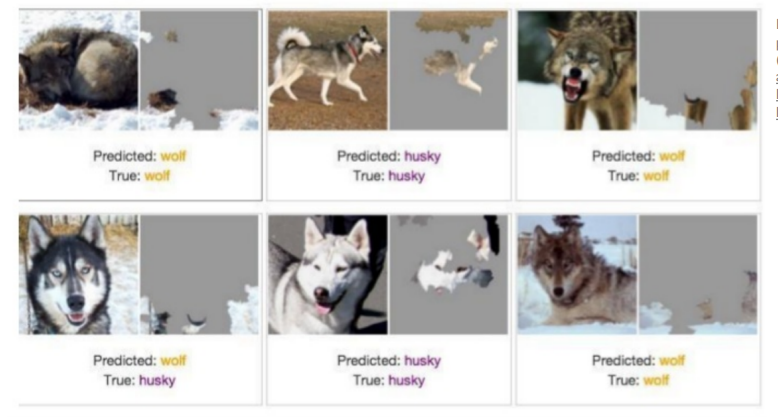
The lack of explainability can lead to situations where the model assigns a higher weight to those input variables that objectively should not have such a weight.
Example: A review of the solutions of a model that was supposed to classify wolves and huskies showed that it based its conclusions on the fact of the presence of snow in the background (Fig. 10).
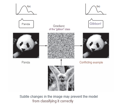
Attackers can add small distortions to images that will not affect a person’s decision, but can confuse an algorithm that has previously proven its effectiveness on images that have not been artificially altered (Fig. 11).
The ethical issues associated with the operation of black box models arise from their tendency to inadvertently make unfair decisions based on sensitive factors such as a person’s race, age, or gender. Example: THE COMPAS system for assessing the risk of re-committing criminal acts adopted race as one of the important characteristics for deciding on a high risk of recurrence.
Interpreted models
Explainability can be considered at all stages of AI development, namely: before modeling, during model development and after modeling.
The easiest way to achieve interpretability is to use only a subset of the algorithms that create interpreted AI models. Linear regression, logistic regression, and the decision tree are commonly used interpreted AI models.
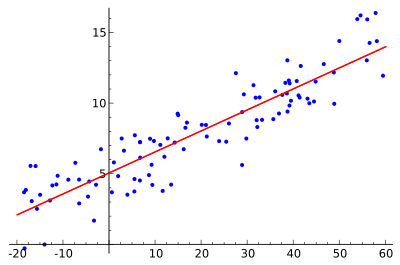
The linear regression model predicts the target as a weighted sum of the input parameters. The linearity of established relationships makes interpretation easier. Linear regression models have long been used by statisticians, computer scientists, and others dealing with quantitative problems.
Linear equations have an easy-to-understand interpretation at the modular level (at the level of weights). Linear models are widespread in medicine, sociology, psychology, etc.
The relationships of the AI model must conform to certain assumptions, namely linearity, normality, homoscedasticity (have a constant average variance), independence, fixed characteristics, and lack of multicollinearity.
However, linear models have the following disadvantages. Each nonlinearity or interaction must be created manually and explicitly passed to the model as an input characteristic; in terms of relationships, linear models are very limited and usually greatly simplify reality, which affects their forecasting capabilities; interpreting the weights can be difficult to understand because the relationship is traced throughout the model. A feature with a high positive correlation with a y result and another trait can gain negative weight in a linear model because, given another correlated trait, it negatively correlates with y in multidimensional space. Fully correlated functions make it impossible to find a one-to-one solution to a linear equation.
Logistic regression models the probabilities of classification problems with two possible outcomes, and is an extension of the linear regression model for classification problems. The interpretation is more complex compared to linear regression because the interpretation of the weights is multiplicative rather than additive.
Logistic regression can suffer from complete separation. If there is a function that perfectly separates the two classes, the logistic regression model can no longer be trained because the weight for that function will not converge—the optimal weight will be infinite.
The advantage of logistic regression in classification problems is that it gives probabilities of obtaining results for a class. This directly leads to its practical significance – it is a powerful statistical method for predicting events that are the result of one or more independent variables.
The model can be extended to predict multiple classes, then it is called polynomial regression.
General linear models (GLM) extend the capabilities of the linear regression model. These models make it possible to use response variables with a different error distribution than normal. GLM is a general mathematical framework for expressing relationships between variables that can express or test linear relationships between a numerical dependent variable and any combination of categorical or continuous explanatory variables. Most teacher-assisted machine learning techniques extend GLM in some way (through penalty methods, ensemble method, combining predictions from multiple machine learning models into a single dataset, and others).
A generalized additive model (GAM) is a generalized linear model in which a linear predictor is linearly dependent on unknown smooth functions of some predictor variables, and interest is focused on inferring about these smooth functions. In its work, GAM uses spline functions , functions that can be combined to approximate arbitrary functions. GAM introduce penalties for scales to keep them close to zero, which effectively reduces the flexibility of splines and reduces the possibility of retraining. The smoothness setting, which is typically used to control curve flexibility, is then adjusted by cross-checking.
Most modifications of the linear model make the model less interpreted. Any communication function that is not an identity function complicates interpretation; interactions also complicate interpretation; the effects of nonlinear functions are either less intuitive or can no longer be summed into a single number. GLM, GAM, and other extensions rely on assumptions about the data generation process. If the assumptions don’t work, the interpretation of the scales no longer works.
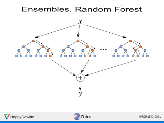
The performance of tree ensembles, such as a random forest or gradient tree, is in many cases higher than that of the most complex linear models.
The ensemble method is based on machine learning algorithms that generate many classifiers and separate all objects from newly arrived data based on their averaging or voting results. Initially, the ensemble method was a special case of Bayesian averaging, but then became more complicated by additional algorithms:
- boosting – converts weak models into strong ones by forming an ensemble of classifiers (improving intersection);
- bagging – collects complex classifiers, while simultaneously training the basic ones (improving unification);
- correction of output coding errors.
The ensemble method is a more powerful tool compared to free-standing forecasting models:
- minimizes the impact of randomness by averaging the errors of each base classifier;
- reduces variance;
- excludes going beyond the set: if the aggregated hypothesis is outside the set of basic hypotheses, then at the stage of the formation of the combined hypothesis it expands by one way or another, and the hypothesis is already included in it.
A decision tree is a decision support method based on the use of a tree graph: a decision-making model that takes into account their potential consequences (with the calculation of the probability of occurrence of an event), efficiency, and resource consumption. The advantages of the method are that it structures and systematizes the problem; the final decision is made on the basis of logical conclusions.
Rice. 14. Decision Tree
Naïve Bayesian classifiers refer to a family of simple probabilistic classifiers based on Bayes’ theorem, which treats functions as independent (this is called a strict, or naïve, assumption). Used in the following areas of machine learning: detection of spam coming to e-mail; automatic linking of news articles to thematic headings; identification of the emotional coloring of the text; recognition of faces and other patterns in images.
The RuleFit algorithm studies a sparse linear model with original functions, as well as a number of new functions that are the rules of decision-making. The new functions reflect the interaction between the original functions. RuleFit automatically generates these functions from decision trees. Each path through the tree can be transformed into a decision rule by combining split decisions into a rule. Decision trees in this case are trained to predict the outcome of interest, which ensures that a partition is needed for the prediction problem. For RuleFit, you can use any algorithm that generates multiple decision trees, such as a random forest (See Figure 15).
Each tree is broken down into decision rules, which are used as additional functions in the sparse linear regression model. RuleFit has a feature importance metric that helps you identify linear conditions and rules that are important for predictions. The importance of the function is calculated based on the weights of the regression model. The importance score can be aggregated for the original functions. RuleFit also presents partial-dependency graphs to show the average forecast change as the characteristic changes.
The k-nearest neighbors method is used for classification tasks (sometimes in regression problems), the object belongs to the class to which most of its neighbors belong (Fig. 16).
In the learning process, the algorithm simply remembers all the feature vectors and their corresponding class labels. When working with real data, i.e. observations whose class marks are unknown, the distance between the vector of the new observation and previously remembered ones is calculated. Then, k of the nearest vectors to it is selected, and the new object belongs to the class to which most of them belong.
Increasing the value of the k parameter increases the validity of the classification, but the boundaries between classes become less clear. In practice, heuristic methods for selecting the k parameter, for example, cross-checking, give good results.
Despite its relative algorithmic simplicity, the method shows good results. The main drawback: high computational labor intensity, which increases quadratically with the increase in the number of training examples.
Posteriori methods of explanation
When machine learning models do not meet any of the criteria imposed to declare them transparent, a separate method must be developed and applied to the model to explain its solutions. This is the goal of posteriori explanatory techniques, which aim to convey understandable information about how an already developed model produces its predictions for any given input.
The interpretation in these methods is based on limited access to the inner workings of the model. For example, explanations can be derived from gradients, “running” the model in the opposite direction, or by querying by evaluating simpler surrogate models to capture the observed local input-output behavior.
Global a posteriori explanations are useful for decision-makers who are supported by a machine learning model. Doctors, judges, and loan officers get a general idea of how the model works, but there is bound to be a gap between the black box model and the explanation. Local a posteriori explanations are relevant to individuals, such as patients, respondents, who are influenced by the outcome of the model and who need to understand its interpretation from their specific point of view.
A great advantage of model-independent interpretation methods compared to model-specific interpretation methods is their flexibility.
Desirable aspects of a model-independent explanatory system are: model flexibility (the interpretation method can work with any machine learning model, such as random forests and deep neural networks); flexibility of explanations (various forms of explanations, for example, a linear formula for some cases, a graph with the importance of functions for others); flexibility of representation (the explanatory system should be able to use another representation of the object as an explainable model).
LIME (Local interpretable model-agnostic explanations) explains the classifier for a particular single output of a function and is therefore suitable for local consideration. Explains the individual predictions of a neural network by approximating it locally using interpreted models such as linear models and small trees.
To explain the algorithm solution locally for a particular input, the linear model is trained to simulate the algorithm only for a small area around the input. This linear model, by its very nature, can be interpreted and tells how the output will change if any input function changes.
LIME works with tabular data, text, and images.
Explanations created using local surrogate models can use other (interpreted) functions that the original model was trained with. These interpreted functions must be derived from data instances. A text classifier may rely on embedding abstract words as features, but the explanation may be based on the presence or absence of words in a sentence. A regression model can rely on an uninterpreted transformation of some attributes, but explanations can be created using the original attributes. For example, a regression model can be trained on the components of the method of the main components of survey responses, and LIME can be trained on the original survey questions. Using interpreted functions for LIME can be a great advantage over other methods, especially when the model has been trained with uninterpreted functions.
Model-independent perturbation-based methods (such as LIME) are more prone to instability than their gradient-based counterparts.
In the event of a repeat sampling process, explanations may change. Instability in this case means that the explanations are difficult to trust, and you need to be very critical.
Local surrogate models with LIME are very promising. But this method is still under development, and many problems need to be solved before it can be safely applied.
SHAP (Shap’s Additive Explanation) is a method of explaining individual predictions. SHAP is based on the game of theoretically optimal Shapley values. SHAP defines the marginal contribution of each function to the achievement of the output value, starting with the base value.
Shapley values consider all possible predictions using all possible combinations of input data. With this approach, SHAP can guarantee consistency and local accuracy.
SHAP works well for classification and regression tasks, but is poorly applicable for reinforcement learning.
SHAP has a solid theoretical foundation in game theory. The prediction is fairly distributed among the feature values. At the output, you can get contrasting explanations that compare the resulting forecast with the average forecast.
A quick calculation allows you to calculate the set of Shapley values required to interpret the global model. Global interpretation techniques include the importance of characteristics, characteristic dependence, interactions, clustering, and summary graphs. With SHAP, global interpretations are consistent with local explanations, since Shapley values are the “atomic unit” of global interpretations.
Disadvantages of the method:
- The problem of slow solutions (SHAP methods require the calculation of Shap values for multiple values) remains relevant to global explanations of the model.
- SHAP can ignore function dependencies when replacing feature values with random values, which in turn can cause too much value to unlikely data points.
TreeSHAP solves the problem of extrapolation to unlikely data points, but creates a new problem. TreeSHAP modifies the function of the truth value based on a conditional expected prediction. If you change a function that does not affect the prediction, the values may return a value other than zero.
LIME and SHAP were recognized by the scientific community as the most promising models of a posteriori explanations that do not depend on the model, but a group of scientists conducted a study that proved that these methods poorly determine the bias of the model. In an experiment with a specially created classifier, which was clearly biased, using only data on the race of a person as significant features, these methods ignored bias, finding quite innocuous explanations for the output data obtained during the work of the model.
Explanations of these classifiers generated using out-of-the-box implementations of LIME and SHAP do not mark any important sensitive attributes (e.g., race) as important classifier features for any of the test cases, demonstrating that biased classifiers have successfully deceived these methods of explanation.
The other two closely related branches of interpretability methods are the backpropagation approaches and the gradient-based approaches. They either propagate the algorithm’s solution back across the model or use the sensitivity information provided by the loss gradients. Examples include deconvolution networks, controlled backpropagation, Grad-CAM, integrated gradients, and layer-by-layer reverse propagation (LRP).
GradCAM is a layer attribution method developed for convolutional neural networks and usually applied to the last convolutional layer. GradCAM calculates the gradients of a given output parameter in relation to a given layer, averages them for each output channel, and multiplies the average gradient for each channel by activating the layer. The results are summed up across all channels, and the ReLU activation function is applied to the output, which returns only non-negative attributes.
GradCAM is often used as a common attribution method. To do this, the GradCAM attributes are subjected to upscaling sampling and treated as a mask for the input data, since the output of the convolutional layer usually spatially coincides with the input image.
Many of these approaches have been developed only for (convolutional) neural networks. A notable exception is LRP.
Layer-wise relevance backpropagation (LRP) is a technique that identifies important pixels by performing a back pass in a neural network. A reverse pass is a conservative procedure for redistributing relevance, in which the neurons that contribute the most to a higher level receive the most relevance from it.
The method can be easily implemented in most programming languages and integrated into existing neural networks. The propagation rules used by the LRP can be understood as a deep Taylor decomposition for many architectures, including Deep Sparse Rectifier Neural Networks or LSTM.
LRP also works great for convolutional neural networks (CNNs) and can be used for long short-term memory (LSTM) networks.
In the Integrated Gradients (IG) method, the gradient of the prediction output is calculated based on the characteristics of the input data along the integral trajectory. The purpose of the method is to explain the relationship between the predictions of the model in terms of its characteristics. Usage: Understand the importance of functions, determine data skew, and debug model performance.
IG has become a popular method of interpretability because of its wide applicability to any differentiable model, ease of implementation, theoretical justification, and computational efficiency compared to alternative approaches, allowing it to be scaled to large networks and functions.
This method does not require modification of the source network, is easy to implement and is applicable to many deep models (sparse and dense, text and visual).
Integrated gradients define the importance of functions in individual examples, but do not provide a visualization of the importance of functions for the entire dataset; define the individual values of functions, but do not explain interactions and combinations of functions.
Based on the integrated gradient method, the XRAI method evaluates overlapping areas of the image to create a significance map that highlights the corresponding areas of the image rather than the pixels (Figure 17).
Regardless of pixel-level attribution, XRAI super-segments the image to create a patchwork quilt of small areas. XRAI uses a graph method to create image segments. Attribution is then aggregated at the pixel level in each segment to determine its attribution density. Using these values, XRAI ranks each segment and then orders the segments from most positive to least positive. This determines which areas of the image are most noticeable or most strongly influence class prediction.
The method is recommended for natural images, which are any real-world scenes containing multiple objects.
DeepLIFT is a reverse propagation-based approach that attributes modification to input data based on differences between the input data and the corresponding references (or baselines) for nonlinear activations. Thus, DeepLIFT attempts to explain the difference between the raw data and the reference data in terms of the difference between the input data and the reference data.
DeepLIFT SHAP is a method that extends DeepLIFT to approximate SHAP values. DeepLIFT SHAP takes the baseline distribution and calculates the DeepLIFT attribution for each pair of input data and baselines and averages the resulting attributions for each sample input.
DeepLIFT rules for nonlinearities serve to linearize nonlinear network functions, the method approximates SHAP values for a linearized version of the network. The method also assumes that the input functions are independent.
Existing solutions for XAI
IBM’s AIX360 is an extensible set of tools that offers a number of options for improving model explainability. The corresponding Python AI Explainability 360 package includes algorithms covering various metrics of explanations along with intermediary metrics of explainability, and provides tools for visually investigating the behavior of trained models with a minimum amount of code.
The toolkit includes a series of interpretability algorithms that mirror current research on the topic, as well as an intuitive user interface that helps you understand machine learning models from different perspectives. One of the main contributions of AI Explainability 360 is that it doesn’t rely on a single form of machine learning model interpretation. AI Explainability 360 provides different explanations for different roles, such as data scientists or business stakeholders. The explanations generated by AI Explainability 360 can be based on data or on models.
Developers can start using AI Explainability 360 by including interpreted components using the APIs included in the toolbox. AI Explainability 360 includes a series of presentations and tutorials that can help developers get started relatively quickly.
The interpretability of a model in Microsoft Azure is provided by an SDK that can explain model predictions by generating the importance of function value for the entire model or individual data points, and by using interactive visualization to discover relationships in the data and explanations during model training.
Azureml-interpret uses interpretability techniques developed in Interpret-Community, an open-source Python package to train interpreted models and help explain black-box AI systems. Interpret-Community serves as the basis for the supported explanatory models of this SDK and currently supports the following interpretability methods: SHAP variations (TreeSHAP, SHAP deep Explainer, SHAP Kernel explainer, etc.), Global Surrogate1, Permutation Feature Importance Explainer2. To explain the operation of deep neural networks, you can use TabularExplainer, which uses SHAP methods.
Google Cloud’s AI Explanations aims to use AI explanations to simplify model development, as well as explain the behavior of the model to key stakeholders. AI Explanations work with models that solve classification and regression problems, demonstrating how a particular data function affected the result. AI Explanations uses the following methods: Integrated Gradient Method, XRAI, and Sampled Shapley. What-If Tool is used for visualizations.
In 2018, the PAIR Team (People + AI Research, part of Google AI) introduced what-If Tool– a tool for detecting bias in artificial intelligence models. It comes as part of the TensorBoard web application. What-If Tool visualizes the impact of certain data on the prediction of the model while being available to those who are not versed in programming.
What-If Tool allows you to:
- Automatically visualize a dataset using Facets. Facets Overview gives you an idea of the form of each function of the dataset; Facets Dive with the help of visualization allows you to study individual observations.
- Edit individual examples from the set and track how this affects the results.
- Automatically create partial dependency graphs that reflect changes in model prediction when a single property changes.
- Compare the most similar examples from the dataset, for which the model gave different predictions.
You can check the operation of the tool on pre-trained algorithms: multiclass classification models; Image classification models regression model. What-if-tool can work with text, visual and tabular data.
The Thales XAI platform provides different levels of explanation, for example, based on examples, based on functions, counterfacts using textual and visual representations, but it is worth noting that the emphasis is on explanation based on semantics using knowledge graphs. Knowledge graphs are used to encode a better representation of the data, structure the machine learning model in a more interpreted way, and adopt semantic similarities for local (instance-based) and global (model-based) explanations.
The explanation of any prediction of the relationship is obtained by identifying representative hotspots in the knowledge graph, that is, the related parts of the graphs that, when removed, adversely affect the accuracy of the prediction.
ELI5 is a Python package that helps you debug machine learning classifiers and explain their predictions. It provides support for multiple machine learning frameworks and packages:
scikit-learn. Currently, ELI5 allows you to explain the weights and predictions of scikit-learn linear classifiers and regressors, print decision trees in text or SVG graphical format, show the importance of functions, and explain predictions of decision trees and tree-based ensembles.
Pipeline and FeatureUnion are also supported.
Functions of some tools in Eli5:
XGBoost — show the importance of functions and explain the predictions of XGBClassifier, XGBRegressor and xgboost. Booster.
LightGBM – Show the importance of functions and explain the predictions of LGBMClassifier and LGBMRegressor.
CatBoost — show the importance of the CatBoostClassifier and CatBoostRegressor functions.
Keras – Explain the predictions of image classifiers using GradCAM visualizations.
ELI5 also implements several algorithms for checking black box models:
TextExplainer allows you to explain the predictions of any text classifier using the LIME algorithm. There are also utilities for using LIME with non-text data and arbitrary black box classifiers, but this feature is currently experimental.
The importance redistribution method can be used to calculate the significance of features for black box evaluators.
It is possible to get a text explanation to display on the console, an HTML version embedded in IPython Notepad or a web panel, a JSON version that allows you to implement custom rendering and formatting on the client, and to convert explanations into pandas DataFrame objects.
Open source packages have greatly improved the reproducibility of research and have made significant contributions to recent research in deep learning and XAI.
Some XAI software packages available on GitHub include:
Interpret from InterpretML can be used to explain black box models and currently supports explainable boosting, decision trees, decision rule list, linear logistic regression, SHAP kernel explainer, TreeSHAP, LIME, Morris sensitivity analysis, and partial dependency.
The IML package covers techniques such as function importance, partial dependency graphs, individual conditional expectation graphs, accumulated local effects, tree surrogates, LIME, and SHAP.
The DeepExplain package includes various gradient-based methods such as significance maps, integrated gradients, DeepLIFT, LRP, etc., as well as perturbation-based methods such as occlusion, SHAP, etc.
Problems related to the development and use of XAI
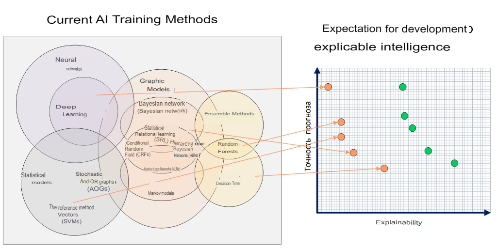
In scientific studies on explainable artificial intelligence, one of the main problems in the development of XAI is the fact that the creation of a more understandable machine learning model can ultimately worsen the quality of its decisions.
It’s not always true that more complex models are inherently more accurate. This statement is incorrect in cases where the data is well structured, and the functions available to the developer are of high quality and value. This case is common in some industry environments because the functions analyzed are limited to controlled physical problems in which all functions are strongly correlated, and not much of a possible landscape of values can be explored in the data.
More complex models have much more flexibility than their simpler counterparts, allowing for the approximation of more complex functions.
The approximation dilemma is closely related to interpretability: explanations made for a machine learning model must meet the requirements of the audience for which they are formed, ensuring the representativeness of the model under study without unnecessarily simplifying its main features.
In science, there are no single objective indicators of what exactly is a good explanation for XAI. To solve this problem, the researchers propose to conduct a series of experiments in the field of human psychology, sociology or cognitive sciences to create objectively convincing explanations.
Explanations are more compelling when they are restrictive, which means that a precondition for a good explanation is that it not only indicates why the model made decision X, but also why it made decision X rather than decision Y. Cause-and-effect relationships are more important for explanations than determining probability. It is necessary to transform probabilistic results into qualitative concepts containing cause-and-effect relationships. It may be sufficient to focus solely on the root causes of the decision-making process. In a number of studies, it has been proven that the use of counterfactual explanations can help the user understand the solution of the model.
Although explanatory methods are increasingly being used as health checks during the development process, there are still significant limitations on existing methods that do not allow them to be used to directly inform end users. These limitations include the need to evaluate explanations by domain experts, the risk of false correlations reflected in the model’s explanations, a lack of causal intuition, and a delay in calculating and displaying explanations in real time. Future studies should seek to address these limitations.
0 Comments